Stairmand High-Efficiency Cyclone

A cyclone is a common piece of industrial equipment that has been used since the 1800s to separate pollutants from gas streams. Its popularity stems primarily from its simple design and low capital and maintenance costs. The Stairmand High-Efficiency Cyclone is a popular industrial cyclone design. Stairmand (1951) proposed a reverse-flow cyclone separator design that combines high separation efficiency with low pressure loss. This cyclone design will be used for this simulation.

The working principle of a cyclone separator is as follows: a vortex is created in a reverse-flow cyclone separator by placing a tangential inlet at the top of the cylindrical part of the cyclone body. The larger and denser part of the dispersed phase is forced outward by centrifugal force and collides with the cyclone wall. The flow near the wall is downward-directed and serves as the driving force for transporting the dispersed phase to the collection reservoir located at the cyclone’s base. At the cone’s bottom, the vortex reverses direction and moves upwards towards the outlet.

Cyclone geometry

Figure 1 depicts the Stairmand High-Efficiency cyclone design, which is based on several ratios calculated using characteristic dimensions normalised by the cyclone diameter. The ratios are shown in the table below. The characteristic dimensions are inlet height $(a)$ , inlet width $(b)$ , cylinder height $(h)$ , total height $(H_t)$ , bottom cone diameter $(B_c)$ , vortex finder diameter $(D_e)$ , and vortex finder length $(S_e)$ . The characteristic dimensions are illustrated in the figure below.

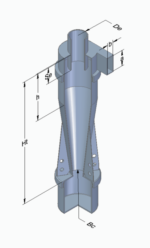
a/D	b/D	$D_e$ /D	$H_t$ /D	h/D	$S_e$ /D	$B_c$ /D
0.5	0.2	0.5	4.0	1.5	0.5	0.375

Grid generation

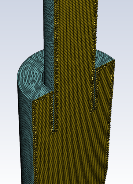
The mosaic grid function in Ansys Fluent is used to discretize the fluid domain. The mosaic grid’s boundary layer contains prismatic elements, while the core contains hexahedral elements. Polyhedrons connect the two types of elements. Ansys Fluent automatically generates a poly-hexacore grid, which reduces the total number of cells used when compared to a standard unstructured grid. The grid is shown below.

Grid independence study

Grid independence is demonstrated by comparing the static pressure at the inlet for grids of varying sizes. A total of three grids of 599,763, 1,492,638 and 3,869,711 cells are analysed. The grids are refined in all directions except the height of the first prism layer nearest the wall, which remains constant. The PRESTO! scheme is used for interpolation of the pressure gradient and the second order upwind scheme for the discretization of all advection terms.
The grid independence study uses Roache’s (1997) grid convergence index (GCI) criteria. The grid refinement ratio between coarse and medium grids is 1.36, while medium and fine grids have a ratio of 1.37. The CGI is calculated using a safety factor of 1.25, as recommended by Roache (1997). The change in grid size results in an uncertainty of less than 1%. This uncertainty is small enough to justify using a grid of 1,492,638 cells.

Turbulence modelling

A major drawback of the standard two-equation RANS turbulence models (such as the $k-\epsilon$ or $k-\omega$ models) is the assumption that the turbulent viscosity (or eddy viscosity) is isotropic. This assumption implies that the turbulence is the same in all directions, which is not always true, especially in flows with strong gradients, such as in a cyclone separator. This assumption can negatively influence the accuracy of the predictions. This can be mitigated by using an anisotropic turbulence model, such as the Reynolds Stress Model (RSM). The RSM resolves the anisotropy of turbulence by solving transport equations for each of the six independent components of the Reynolds stress tensor. Additionally, a transport equation for the dissipation rate of turbulent kinetic energy is used to close the model.

Boundary conditions

The material that was selected fluid is air, with a density of $1.225 kg/m^3$ and a dynamic viscosity of $1.789e-5Pas$ . The inlet’s boundary condition is set at a uniform velocity of $22.66 m/s$ . This velocity corresponds to the Reynolds number used in Hoekstra’s (2000) experiments. The outlet’s boundary condition is set to zero pressure. The turbulent intensity at the inlet and outlet is estimated using the following equation:

$\begin{equation*}T_I=0.16Re_{d_h}^{\frac{-1}{8}}\end{equation*}$

where Re is the Reynolds number calculated using the hydraulic diameter $(d_h)$ . The turbulent length scale is related to the size of the largest energy-containing eddies in the main flow and estimated using:

$\begin{equation*}l=0.07d_h\end{equation*}$

A no-slip condition is imposed on the cyclone’s walls. To maintain an acceptable wall-clock-time for CFD simulations, the standard wall function in Ansys Fluent is used. As a result, the first cell from the wall is placed in the log layer rather than the viscous sublayer. The standard wall function calculates the mean velocity near the wall as follows:

$\begin{equation*}u^* = \frac{1}{\kappa} ln \left( Ey^+ \right)\end{equation*}$

where κ is the Von Kármán constant and E is a constant based on wall roughness. For a smooth wall, E is roughly equal to 9.793. This equation applies to turbulent flows along smooth walls between $30<y^+<300$ . The height of the first prism layer near the wall is defined so that the $y^+$ value ranges between 30 and 60 across the fluid domain.

Solver settings

The following solver settings are used in this simulation:

A transient simulation is resolved because of the vortex core’s transient nature.
Viscous model: RSM Linear pressure strain with standard wall functions
Pressure velocity coupling: PISO after initialization
Gradient: Least squares cell based
Pressure: PRESTO! Large deviations are produced by all other pressure interpolation schemes.
Momentum: Second Order Upwind
Turbulent kinetic energy: Second Order Upwind
Turbulent dissipation rate: Second Order Upwind
Reynolds stresses: Second Order Upwind
Higher Order Term Relaxation enabled
Under relaxation factors: unity for all transport equations

Simulation strategy

The CFD simulation is initiated with a steady-state simulation using the k-epsilon RNG model using the SIMPLEC algorithm for pressure velocity coupling for 2500 iterations using the default under relaxation factors (URF). After this step, the turbulence model is changed to the RSTM and solved for another 5000 iterations. The simulation is then changed into a transient simulation and solved until convergence is reached. The PISO pressure-velocity algorithm is used for the transient simulation with the URF’s set to unity. The time-step is equal to 1e-05s resulting in a maximum Courant–Friedrichs–Lewy (CFL) number of below unity.

Convergence

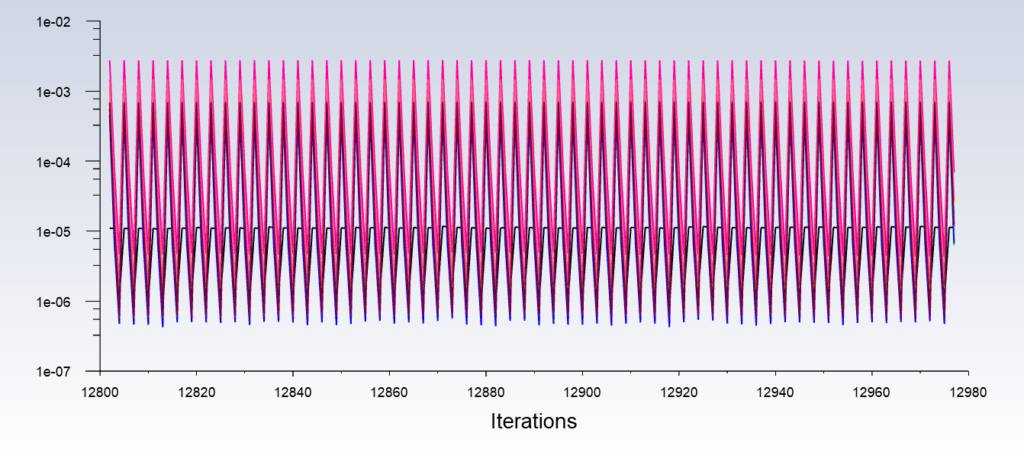
There is a downward trend in the residuals. In five iterations, the threshold of $1e-05$ is reached in each time step.

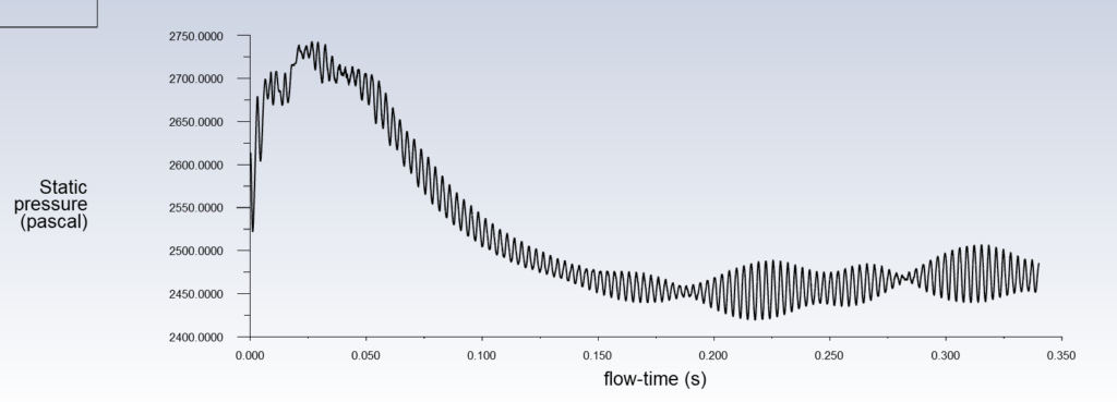
In order to evaluate convergence, the static pressure at the inlet is used. According to the figure below, the final value was obtained after roughly $0.3$ seconds of flowtime. The vortex’s transient behaviour, also known as vortex core precession, is what causes the oscillations in static pressure.

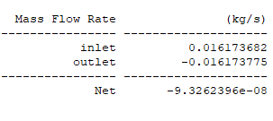
The mass imbalance shows that what is flowing into the computational domain also exits the computational domain. Continuity is therefore guaranteed:

Results

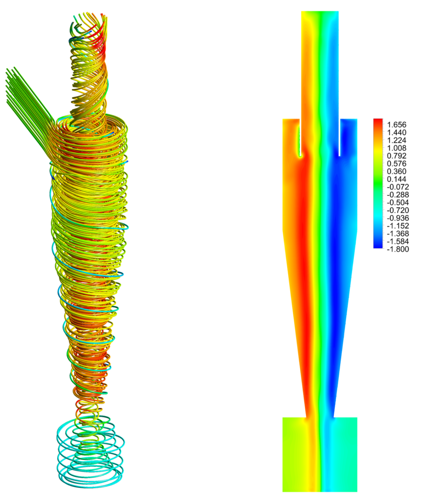
The figure below on the left illustrates the use of streamlines to visualise the general flow profile. The color of the streamlines represents the velocity; red represents the maximum velocity, and blue represents the minimum velocity. These streamlines reveal that an outer and an inner vortex dominate the cyclone’s flow. The outer vortex reverses direction at the bottom of the conical part of the cyclone and exits via the vortex finder on top. The figure below shows the tangential velocity component, normalised with the velocity at the inlet, on the right. The velocity profile is almost symmetrical with respect to the centerline of the cyclone, which is an indication of convergence.

The vortex core is defined as the region where the vortex reaches its maximum tangential velocity, which is approximately the size of the vortex finder. In the Stairmand design, the vortex finder’s diameter is larger than the cone’s bottom diameter. This causes the vortex to collide with the wall at the bottom of the cone, as is illustrated in the figure below on the right. This could result in the entrainment of particles from the boundary layer into the vortex, reducing the overall separation efficiency.

Tangential velocity

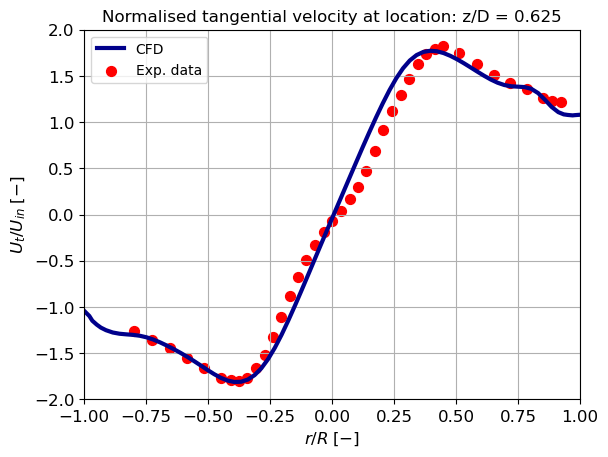
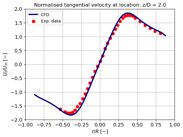
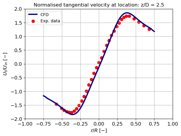
At different cyclone heights, the tangential velocity component is compared with the experimental data from Hoekstra. The graphs below reveal a distinction between a solid body rotation in the core region and a free vortex in the outer region. Both vortices agree well with the experimental data. The magnitude of the tangential velocity in the solid body rotation region, however, is slightly underestimated. The result demonstrates that the RSTM can accurately predict the combined vortex.

The maximum tangential velocity increases at a lower position in the cone. This shows that the magnitude of tangential velocity increases due to a reduction in surface area, and this increase in velocity is larger than the decrease in vortex strength due to wall friction. This can have a positive effect on separation efficiency because the particles experience a larger outward directed force. However, having a high velocity in close proximity to the wall, as previously described, can result in the re-entrainment of separated particles.

Axial velocity

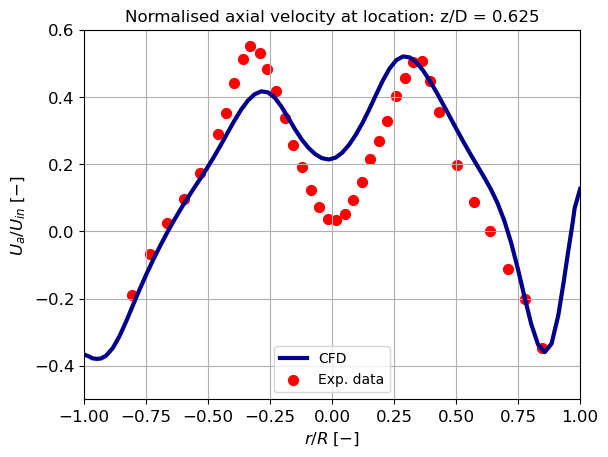
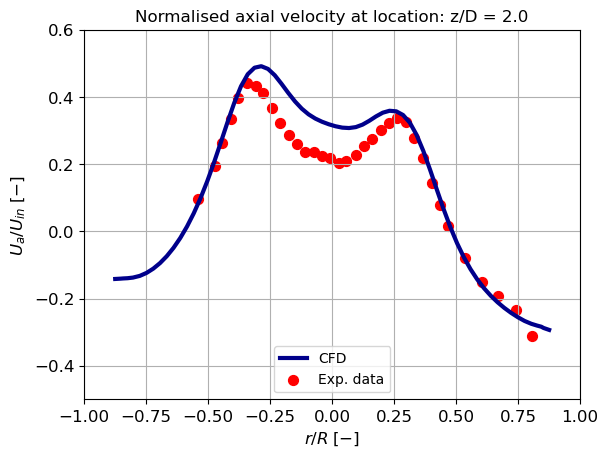
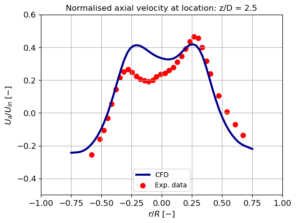
The axial velocity profile can be divided into three regions: the near-wall region, the off-wall region, and the centre region of the vortex. The CFD analysis results, presented below, reveal a deviation in the near-wall region compared to Hoekstra’s experimental results. The left-hand side of the CFD result displays a significant deviation. Using a wall function instead of a finer near-wall grid for wall integration could be the cause of this difference. The wall function may not accurately describe the velocity profile because the cyclone’s velocity profile is more complex than its intended use.

Pressure coefficient

The pressure difference over the cyclone can be calculated by measuring the static pressure at the wall of the inlet and subtracting the static pressure at the wall of the vortex finder (Hoekstra, 2000). The calculation of the static pressure at the inlet of the CFD simulation is straightforward due to the absence of swirl in the inlet channel. However, a strong swirl is present in the vortex finder, resulting a non-uniform static pressure profile. An area-averaged static pressure cannot be used in the outlet because a deviation from the wall static pressure is expected. Therefore, a point measurement is created midway along the vortex finder (location: [0, 0.225, 0.5]) to calculate the time-averaged wall static pressure. A total of time steps is used to calculate the time-averaged static pressure. The calculated pressure difference is converted into a dimensionless loss coefficient by dividing it by the dynamic pressure and compared experimental data. The experimental value is 4.97, while the CFD predicts a loss coefficient of 4.91. The values are in good agreement.

Conclusion

Despite the complexity of the velocity profile in a cyclone, the Reynolds stress turbulence model can accurately describe it. Experimental data exhibits a strong correlation with the result. The near wall area show the largest deviation, which can be corrected by employing an enhanced wall treatment $(y^+~1)$ . Nevertheless, the total computational time will be significantly impacted by this due to the transient nature of the flow and the high Reynolds number.