Natural convection in an enclosed cavity

Natural convection in enclosed cavities is a classic problem in heat transfer, where temperature differences drive fluid motion without any external pumping. This mechanism is not only of academic interest but also central to many engineering applications, from building ventilation and solar collectors to electronic cooling and passive safety systems in nuclear reactors. Despite its apparent simplicity, accurately predicting turbulent natural convection remains a demanding test for CFD methods. A well-documented benchmark for this type of flow is the tall closed cavity experiment performed by Betts and Bokhari, where one vertical wall was heated and the opposite wall cooled.

This study used a two-dimensional CFD simulation to replicate the Betts and Bokhari setup, with the goal of evaluating how accurately the solver could reproduce the characteristic temperature profile observed in the experiment.

Geometry

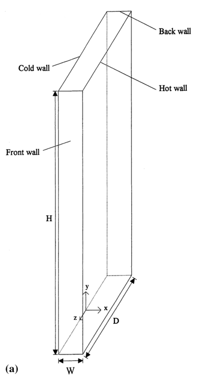
The geometry of the case is a two-dimensional tall rectangular cavity with a height of 2180 mm and a width of 76 mm. The left vertical wall is cooled while the right wall is heated, creating a buoyancy-driven circulation within the enclosure. The cavity is fully closed at the top and bottom.

Grid generation

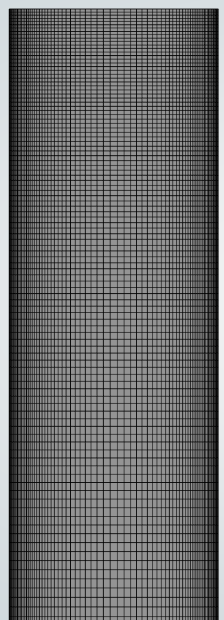
A structured grid was generated to discretize the tall cavity. In the horizontal direction, a bias was applied toward the heated and cooled walls to resolve the thin thermal boundary layers with sufficient accuracy. In the vertical direction, an additional bias was introduced near the top and bottom boundaries to capture the flow reversal in the corner regions. This ensured that both wall effects and corner circulation zones were represented with adequate resolution.

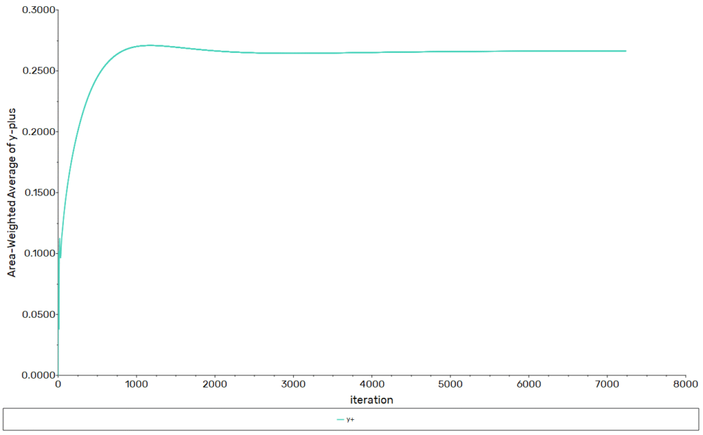
The first cell adjacent to each wall was sized to maintain a $y^+$ value below 1, ensuring that the near-wall gradients were properly captured without reliance on wall functions. The final grid consisted of approximately 37,500 cells, with a maximum aspect ratio of 30 and an orthogonal quality of 1.

Turbulence modelling

To capture the complex transition from laminar to turbulent flow in natural convection, the k–ω SST Transition model (also known as the three-equation transition SST model) was used. This approach extends the standard k–ω SST formulation with additional transport equations for intermittency $(\gamma)$ , making it well suited for predicting boundary-layer transition under varying thermal and flow conditions. In addition, the Kato–Launder production limiter was enabled to prevent over-prediction of turbulence production in regions dominated by buoyancy-driven shear.

Material properties and boundary conditions

Air was modeled as an ideal gas to account for density variations due to temperature differences, which are the driving force behind natural convection. The viscosity was defined using the Sutherland law, while the thermal conductivity was specified as a linear function between the values at 10 °C and 40 °C, temperatures that span the operating range of the problem.

Boundary conditions followed the reference experiment. The left wall was cooled to 15.1 °C, while the right wall was heated to 34.7 °C. The top and bottom walls were treated as adiabatic, ensuring that heat transfer occurred only through the opposing vertical boundaries. These settings replicate the experimental configuration and create the buoyancy-driven circulation that defines the flow in the tall cavity.

Solver settings

The following model and solver settings are selected:

Steady state pressure based solver
Viscous model: $k-\omega$ transition SST with the Kato-Launder production limiter enabled
Pressure velocity coupling: SIMPLEC
Gradient: Green-Gauss Node Based
Pressure: Body Force Weighted
Density: QUICK
Momentum: QUICK
Intermittency: QUICK
Turbulent kinetic energy: QUICK
Turbulent dissipation rate: QUICK
Energy: QUICK
Higher Order Term Relaxation enabled
Under relaxation factors: $P=0.3$ , $U,V=0.2$ , $k, \omega=0.5$ , and $\gamma=0.6$
Initialization: Standard

Convergence

Convergence was assessed by monitoring the residual behavior, selected quantities of interest, and overall energy conservation. The residuals showed a monotonic decline and approached the prescribed threshold values.

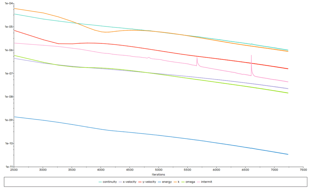
Te graphs below reveal that the final value ahas been reached within 4000 iteration.

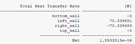
The heat balance confirms that the thermal energy entering the domain through the heated wall is equal to the energy leaving through the cooled wall. This indicates that the conservation of energy is well satisfied in the simulation.

Results

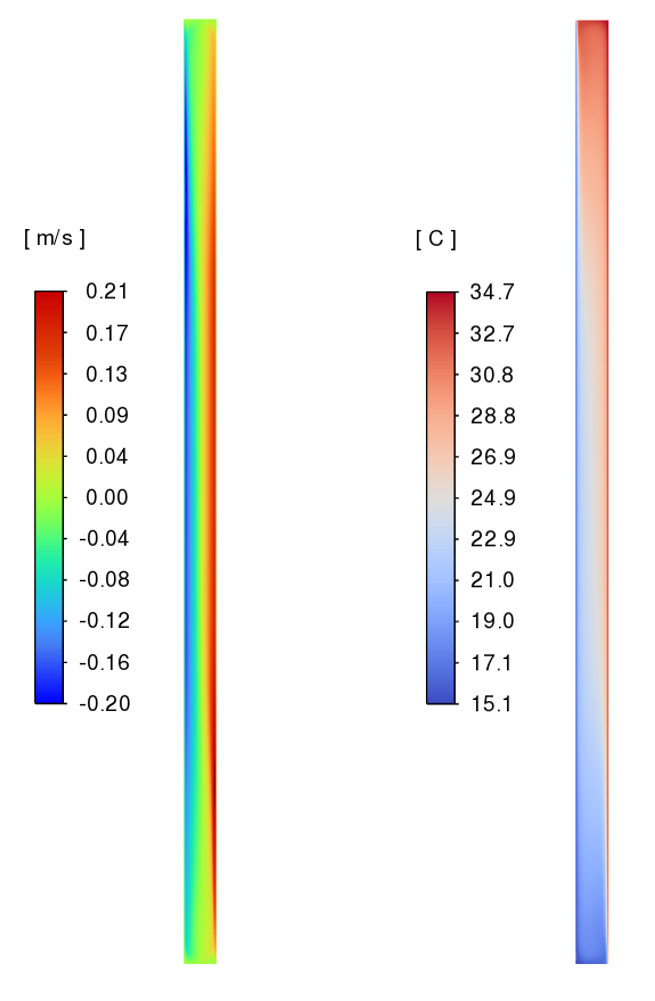
The simulation reveals the characteristic flow and temperature distribution inside the tall cavity. The velocity field shows upward motion along the heated wall and downward motion along the cooled wall, with weak recirculation near the top and bottom corners. The temperature field captures the thin thermal boundary layers adjacent to the vertical walls and a more stratified core region in the center of the cavity. The imposed wall temperatures of 34.7 °C and 15.1 °C are well preserved, and the gradients are clearly visible, reflecting the strong influence of buoyancy-driven convection.

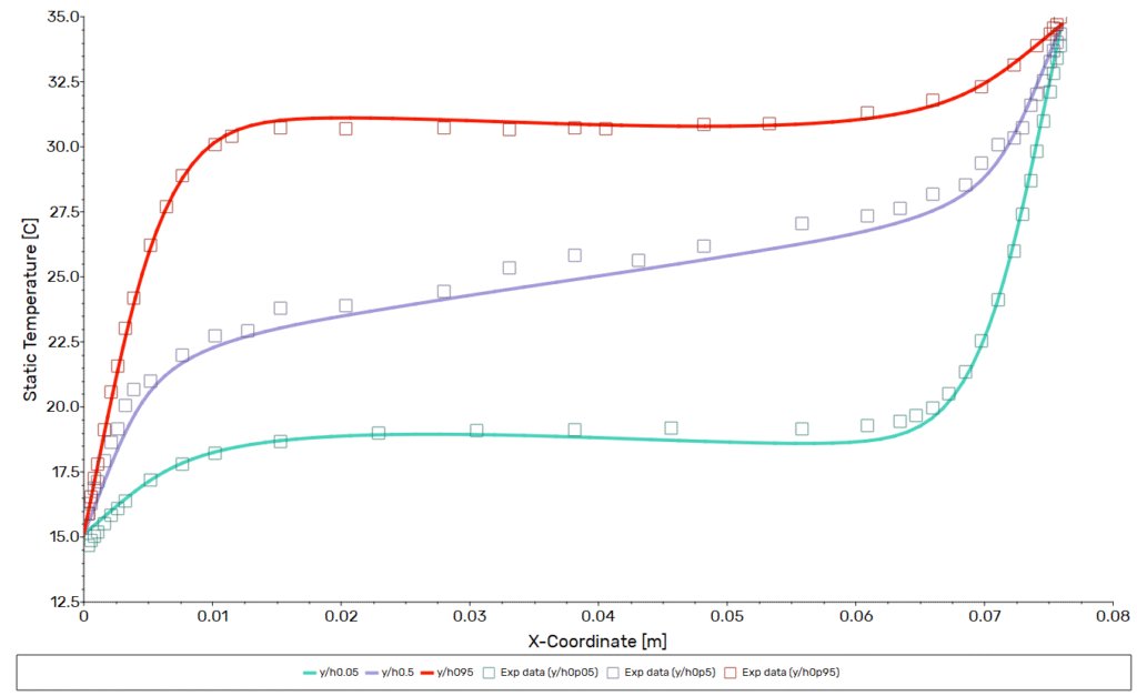
The comparison of simulated and experimental temperature profiles shows very good agreement across the three measured heights. At y/h = 0.05, the CFD solution captures the rapid rise in temperature near the heated wall and the nearly uniform distribution across the core. At mid-height (y/h = 0.5), the predicted profile follows the gradual stratification observed in the experiment. Near the top of the cavity (y/h = 0.95), the simulation successfully reproduces the steep temperature gradients close to the walls, with only minor deviations in the central region. Overall, the results demonstrate that the model accurately captures the thermal boundary layers and the stratified temperature field characteristic of turbulent natural convection in a tall enclosure.

Conclusion

A two-dimensional, wall-resolved RANS setup using the three-equation k–ω SST Transition model provides accurate predictions of turbulent natural convection in a tall cavity. The solver reproduces the thermal boundary layers along the heated and cooled walls as well as the stratified core temperature distribution, showing close agreement with the benchmark data of Betts and Bokhari. Importantly, this is achieved without resorting to excessively fine meshes or high computational cost.

In practical terms, such a setup enables reliable assessment of natural convection performance in enclosed systems where buoyancy-driven flow dominates. This makes it well suited for applications such as building ventilation studies, electronic cooling layouts, and passive safety systems in energy technology. By striking a balance between physical fidelity and computational efficiency, the method delivers trustworthy insights for early-stage design and sensitivity analyses.

The main takeaway is that carefully chosen turbulence models, combined with targeted grid refinement, allow CFD to serve as an effective predictive tool for buoyancy-driven flows.