Vortex shedding is an interesting and well-documented fluid dynamics phenomenon that happens when a fluid flows past a bluff body, such as a cylinder, resulting in alternating low-pressure vortices in the wake. This phenomenon has significant implications for a wide range of engineering applications, including offshore structures, heat exchanger tubes, and tall buildings. Flow past a square cylinder is one of the simplest and most instructive examples of vortex shedding.

This study used a 2D CFD simulation to investigate the vortex shedding behaviour behind a square cylinder with a relatively high Reynolds number of 22,000. Many CFD examinations of bluff body flows are often conducted at lower Reynolds numbers, where flow behaviour is easier to resolve and validate numerically. Higher Reynolds numbers, on the other hand, produce simulation circumstances more similar to those seen in industrial and real-world applications. The purpose of this simulation is to compare the numerical results to current experimental data, focussing on the Strouhal number and wake characteristics.

Geometry

The geometry is simple and clear. It consists of a square cylinder with a length of four centimetres, where the sides of the cylinder will henceforth be referred to as D. A total of 10D is added in front of the domain and 22D behind the domain. The overall height of the fluid domain measures 12D. The domain is divided for meshing purposes.

Meshing

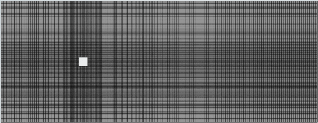
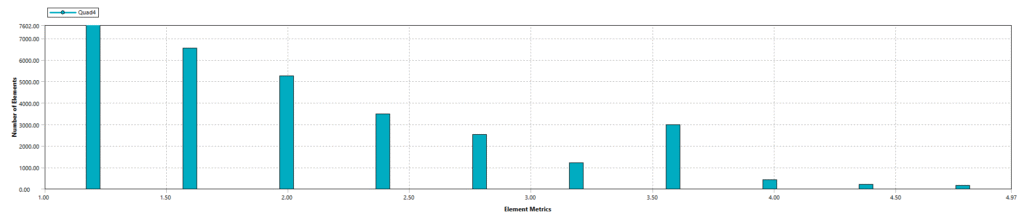
The mesh for this simulation was created to achieve a balance between computational efficiency and the necessary accuracy to effectively capture the unsteady vortex shedding occurring behind the square cylinder. Targeting a Y+ value of about 30 allowed wall functions to be applied in the near-wall area, lowering the total number of cells (~30k cells) while preserving a respectable level of accuracy close to solid borders. This method is often seen in large industrial and civil engineering CFD projects, where fully resolving the boundary layer could result in unreasonable computational costs. Special attention was given to managing the aspect ratio of the cells, since higher aspect ratios in transient, fluctuating flows can lead to numerical diffusion and reduce the accuracy of the solution. In this instance, the maximum aspect ratio was limited to 5 to maintain the integrity of the wake structures (see figure below).

Turbulence modelling

The k-epsilon RNG turbulence model was selected for this simulation, along with the scalable wall function to effectively describe the near-wall region. The RNG (Renormalisation Group) variant was selected instead of the standard and realisable k-epsilon models due to its enhanced accuracy in flows characterised by strong streamline curvature, high strain rates, and swirling effects, conditions that are present in the unsteady wake behind a bluff body at high Reynolds numbers. It is also less diffusive than the standard k-epsilon model, which makes it more effective in capturing complex shear flows. Another significant benefit of the RNG model is its effectiveness in flows with low turbulence intensity regions, such as the wake downstream of the square cylinder. To enhance the physical realism of the simulation, production limiters have been enabled within the turbulence model settings. These limiters assist in avoiding the artificial overproduction of turbulent kinetic energy in areas where numerical instabilities or high strain rates could lead to unphysical outcomes.

Material properties and boundary conditions

The material properties and boundary conditions are chosen so that the Reynolds number equals 22000. In this analysis, water is selected with a density of and a dynamic viscosity of . A uniform velocity of in the X-direction is prescribed at the inlet. The turbulence intensity is set at , consistent with the experiments conducted by Lynn (1995). The viscosity ratio is set at , aligning with Bosch’s recommendation. The outlet is set to outflow.

Solver settings

The following model and solver settings are selected:

• Transient solver
• Viscous model: k- RNG with scalable wall functions, curvature correction, and the Kato-Launder production limiter enabled
• Pressure velocity coupling: PISO
• Gradient: Least squares cell based
• Pressure: PRESTO!
• Density: Second Order Upwind
• Momentum: Second Order Upwind
• Turbulent kinetic energy: Second Order Upwind
• Turbulent dissipation rate: Second Order Upwind
• Transient formulation: Bounded second order implicit
• Higher Order Term Relaxation enabled
• Under relaxation factors equal to unity for all transport equations
• Initialization: Standard with an X-velocity of

Convergence

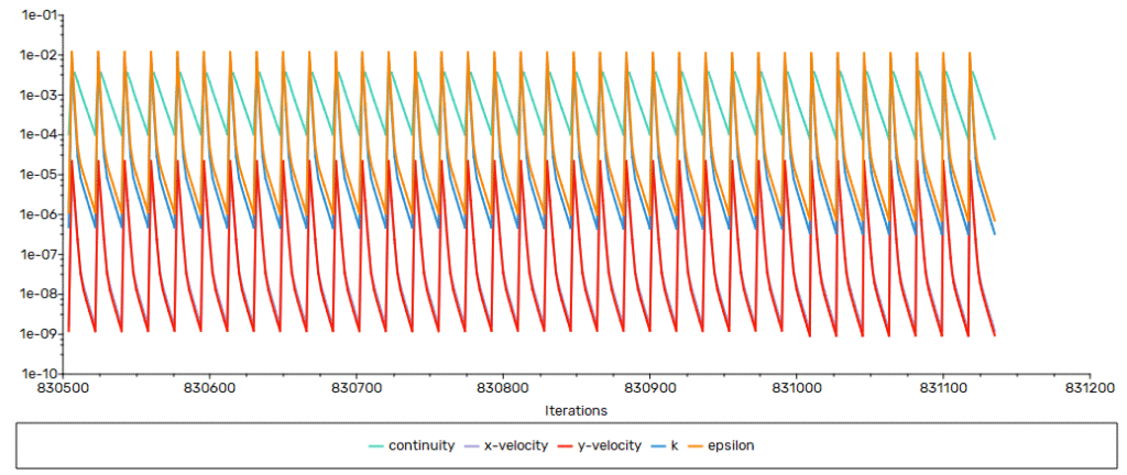
Convergence is evaluated by examining the behaviour of the residuals, ensuring mass conservation, and considering one quantity of interest. Every time-step shows a downward trend in the residuals. The threshold of 1e-05 is attained at each time step.

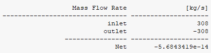
The mass imbalance shows that what is flowing into the computational domain also exits the computational domain. This indicates that the continuity equation is well satisfied.

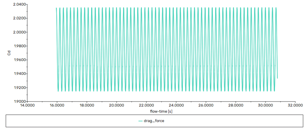
To assess convergence, the drag force of the cylinder is evaluated. The graph below illustrates a consistent pattern of the drag force.

Results

The video below shows the simulation results for the normalized velocity field around the square cylinder at a Reynolds number of 22,000. The alternating vortex shedding in the wake region is clearly visible, with distinct low-velocity zones forming behind the cylinder and being carried downstream.

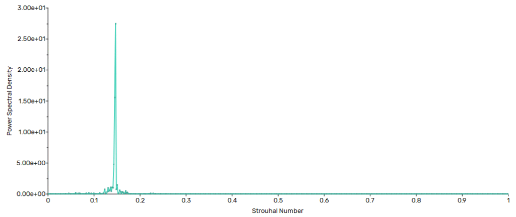
The vortex shedding frequency can be determined by applying a Fast Fourier Transform (FFT) to a time-dependent signal, such as the pressure fluctuations in the wake region. The resulting power spectral density, plotted against the Strouhal number, is shown below. A distinct peak appears at a Strouhal number of 0.14, which is in very close agreement with the experimental results reported by (Lynn, 2006).

The table below presents a comparison between the simulation results and experimental data. The data suggests that the simulation effectively replicates the physics with sufficient accuracy while maintaining a low computational expense.

	Drag coefficient	Strouhal number
CFD simulation	1.97	0.14
Experiment (Lynn, 2006)	2.13	0.13

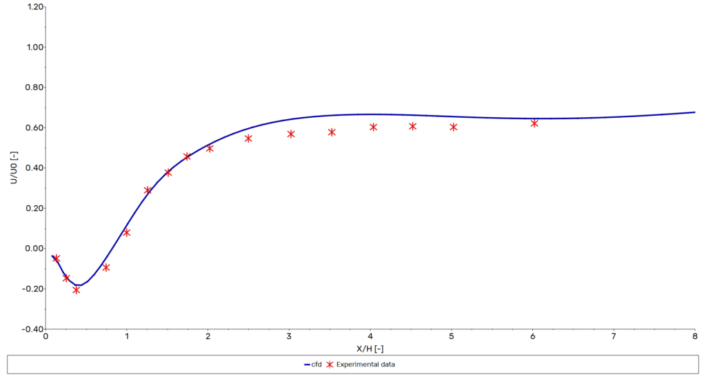
The recovery of the streamwise (X-direction) velocity in the wake of the square cylinder is a key indicator of how well the simulation captures the underlying flow physics. The graph below compares the normalized X-velocity profiles obtained from CFD with experimental data, plotted as a function of dimensionless streamwise distance. The results show very good agreement, with only minor deviations observed in the near-wake region. This suggests that the simulation not only captures the vortex shedding frequency accurately, but also replicates the momentum redistribution in the wake with sufficient fidelity.

Conclusion

This study demonstrates that even a relatively simple two-dimensional CFD simulation using wall functions can effectively capture the key physics of vortex shedding behind a square cylinder at high Reynolds numbers. Despite the use of modeling simplifications, such as scalable wall functions and a coarser mesh, the simulation shows excellent agreement with experimental results in terms of Strouhal number, drag coefficient, and wake velocity profiles.

This approach is particularly well-suited to applications in civil and structural engineering, where computational efficiency is often prioritized over fine-scale turbulence resolution. The ability to achieve reliable results at a low computational cost makes this method highly valuable for preliminary design studies, parametric analyses, and flow assessments in large-scale engineering projects.

Ultimately, the simulation highlights the strength of turbulence models like the RNG k-ε in resolving complex wake dynamics when paired with thoughtful meshing and solver strategies.