NACA-0012 – orangeflow

The National Advisory Committee for Aeronautics (NACA), presently known as NASA, created the symmetric NACA-0012 airfoil shape. This airfoil belongs to the NACA four-digit series. The ’00’ indicates that it is a symmetric airfoil without any camber. The ’12’ indicates that the maximum thickness of the airfoil is 12% of the chord length. The NACA-0012 profile is widely used in aerodynamic research and applications because of its straightforward design and thoroughly documented performance characteristics. The purpose of this study is to conduct a 2D CFD simulation of the NACA-0012 airfoil and compare the results to experimental data.

Geometry

The geometry is created in SpaceClaim using the equation specified on the NASA website:

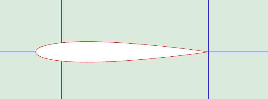
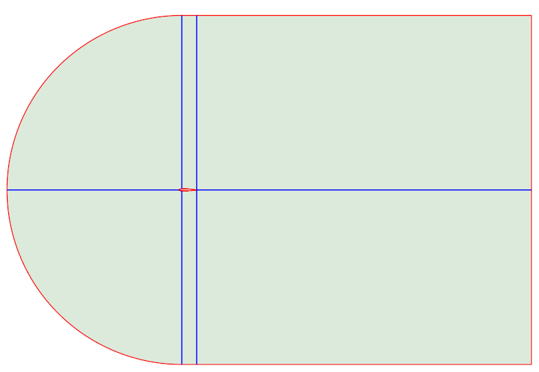
$\begin{equation*}y= - 0.59468918 \left( 0.29822277\sqrt{x} - 0.12712523x - 0.35790791x^2 + 0.29198497x^3 - 0.10517461x^4 \right)\end{equation*}$

The fluid domain is extended 10 chord lengths above and below the chord line to prevent boundary interference. The domain in front of the airfoil extends for a distance of 10 chord lengths to ensure that the flow is fully developed before reaching the airfoil. The domain extends 20 chord lengths behind the airfoil to accurately capture the wake and any flow separation that may occur.

Grid generation

The grid is constructed so that the leading edge of the airfoil aligns with the circular front of the domain, while the sides extend to the sharp trailing edge. This approach ensures optimal distribution of grid points along the airfoil surface, preventing abrupt changes in cell size. A line from the trailing edge to the domain’s end provides sufficient grid resolution in the wake region. Additionally, guide lines perpendicular to the airfoil apply biasing towards the airfoil, ensuring a consistent growth of the boundary layer mesh and maintaining a $y^+$ value of 1.

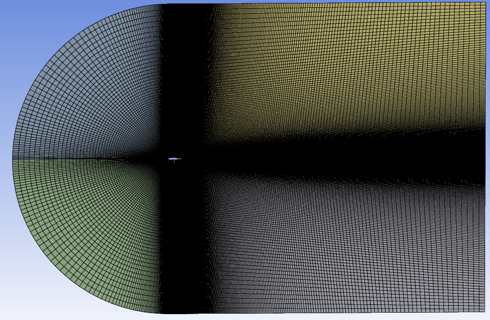
Outside the domain, above and below the airfoil, large variations in cell size are observed. While such differences are typically undesirable, they are permissible here due to the negligible gradients in this region. However, in regions where significant gradient changes are expected, the transitions between cells are made smooth:

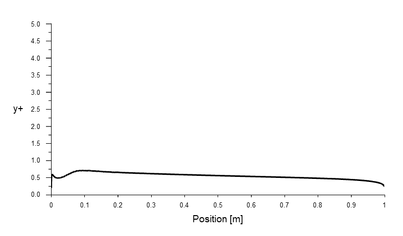
The resolution of the boundary layer grid is sufficient to fully resolve the boundary layer, as shown in the graph below $(\alpha = 0^{\circ})$ , where $y^+$ is plotted as a function of the location on the airfoil. The values are consistently below one.

The first cell adjecent to the airfoil is $4 \mu m$ heigh. Using the bias factor and number of divisions set in the Workbench Mesher, the growth rate can be calculated by using:

$\begin{equation*}r = \left( \frac{a_N}{a_1} \right)^{\frac{1}{N-1}} \approx 1.045\end{equation*}$

Where $a_N$ is the height of the Nth cell, $a_1$ is the first cell height, and $N$ is the total number of divisions. The growth rate $(r)$ corresponds to that used in high-fidelity simulations and remains constant up to the last cell. It is necessary to take into account the maximum aspect ratio in addition to the growth rate. The maximum value in this grid is less than 500 and is located directly adjacent to the airfoil wall.

Grid independence

The grid independence is assessed by comparing the lift coefficient at an angle of attack of $4^{\circ}$ . Three grids, consisting of 169,800, 397,600, and 930,700 cells, are analyzed. The grid convergence index (GCI) criteria of Roache (1998) are adopted for this study. The grid refinement ratio is 1.53 between both the coarse and medium grids and the medium and fine grids. A safety factor of 1.25, as recommended by Roache (1998), is applied in the GCI calculations. The variation in grid size results in an uncertainty of less than 0.25%.

Turbulence model

The Spalart-Allmaras turbulence model was selected for this simulation because it is effective at handling aerodynamic flows, particularly those with adverse pressure gradients. The Spalart-Allmaras turbulence model was formulated by Philippe Spalart and Serge Allmaras, who are affiliated with Boeing. Its primary purpose was to optimise airfoils in the aerospace industry. When it was first introduced, it offered a dependable alternative to other models, such as the k-epsilon model, and it generated positive results in the airfoil and turbine blade applications for which it was calibrated. The model is both robust and computationally efficient, requiring only one transport equation to describe the evolution of the modified turbulent viscosity. However, one of its limitations is its inability to accurately predict free shear flows, such as jet and wake flows.

Material properties

In this simulation, air is used as the fluid. The two most significant material properties are density and viscosity. The ideal gas law is employed for density calculations, while the Sutherland method is used for determining viscosity. Although the Mach number is below 0.3, indicating that the flow can be considered incompressible, there are still slight variations in viscosity and density, on the order of a few percent. Given that this is a 2D simulation, solving an additional transport equation for energy will not significantly increase the total computational time but will increase the accuracy.

Boundary conditions

According to NASA, the Reynolds number for the experiment with tripped data is equal to 6 million, using an airfoil with a chord length of 1 meter at a reference temperature of $300K$ . The Reynolds number is calculated as follows:

$\begin{equation*} Re_c = \frac{\rho U_{\infty} C}{\mu} \quad \rightarrow \quad Re_c = \frac{\rho \cdot \sqrt{\gamma R_s T} \cdot M \cdot C}{\mu} \end{equation*}$

Where $\rho$ is the density in $kg/m^3$ , $\sqrt{\gamma R_sT}$ the speed of sound with $\gamma=1.4$ , $R_s = 287.05$ $J/kgK$ , and $T$ the reference temperature in K. Furthermore, $M$ is the Mach number $(0.15)$ , C the chorde length $(1m)$ , and $\mu$ the dynamic viscosity $(1.8537e-5 \;Pa \cdot s)$ . All values are known except for the density, which can be calculated using the Reynolds number, yielding $\rho = 2.14 \; kg/m^3$ . The total pressure can be calculated using the ideal gas law:

$\begin{equation*}p = \rho R_s T = 184286 Pa\end{equation*}$

A pressure far field boundary condition is appropriate because the boundaries of the computational domain are situated far enough from the airfoil. For this simulation, the far field boundary condition takes the gauge pressure, Mach number, direction of the flow (angle of attack), and static temperature as input values. The gauge pressure is calculated using the total pressure from above:

$\begin{equation*}\frac{p_t}{p_s} = \left[ 1+ \left( \frac{\gamma -1 }{2} \right)M^2 \right]^{\frac{\gamma}{\gamma-1}} \qquad \rightarrow \qquad p_s = 181413Pa\end{equation*}$

The static temperature is calculated using:

$\begin{equation*}\frac{T_t}{T_s} = 1+ \left( \frac{\gamma -1 }{2} \right)M^2 \qquad \rightarrow \qquad T_s = 298.7K\end{equation*}$

The same range of angles of attack as used in the experiments will be applied. The turbulence viscosity ratio is set to a value of 1.2 for all simulations, as obtained from NASA.

The other boundary condition is the airfoil surface. This boundary condition is treated as an adiabatic wall with a no-slip condition enforced.

Solver settings

The following model and solver settings are selected:

Viscous model: Spalart-Allmaras with curvature correction enabled
Energy equation enabled
Pressure velocity coupling: Coupled (converged faster than a segregated solver)
Gradient: Green-Gauss Node Based (more accurate than the default least squares cell based)
Pressure: Second order
Density: Second Order Upwind
Momentum: Second Order Upwind
Modified turbulent viscosity: Second Order Upwind
Energy: Second Order Upwind
Higher Order Term Relaxation enabled
Default under relaxation factors
Pseudo time step enabled: time scale factor 1
Length scale method: User-specified 1m (chord length)
Initialization: Hybrid

Convergence

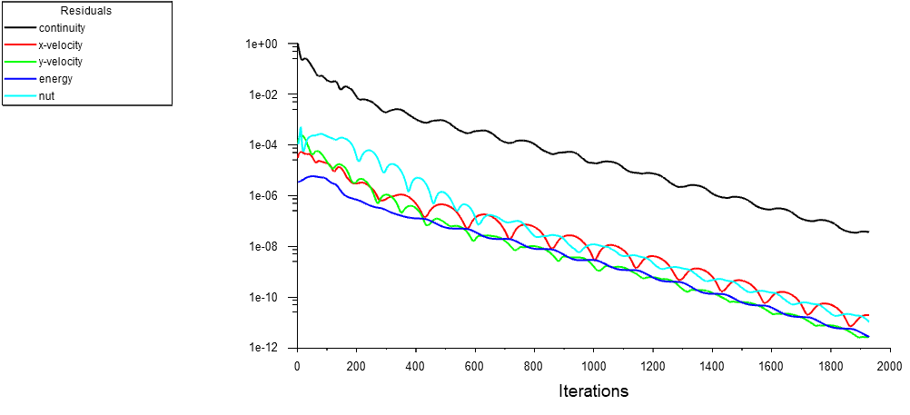
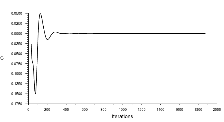
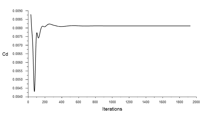
Convergence is assessed by checking the residual behavior and two quantities of interest. The residuals exhibit a monotonic decline and approach the limits of computer accuracy.

Te graphs below reveal that the final value ahas been reached within 800 iteration.

Results

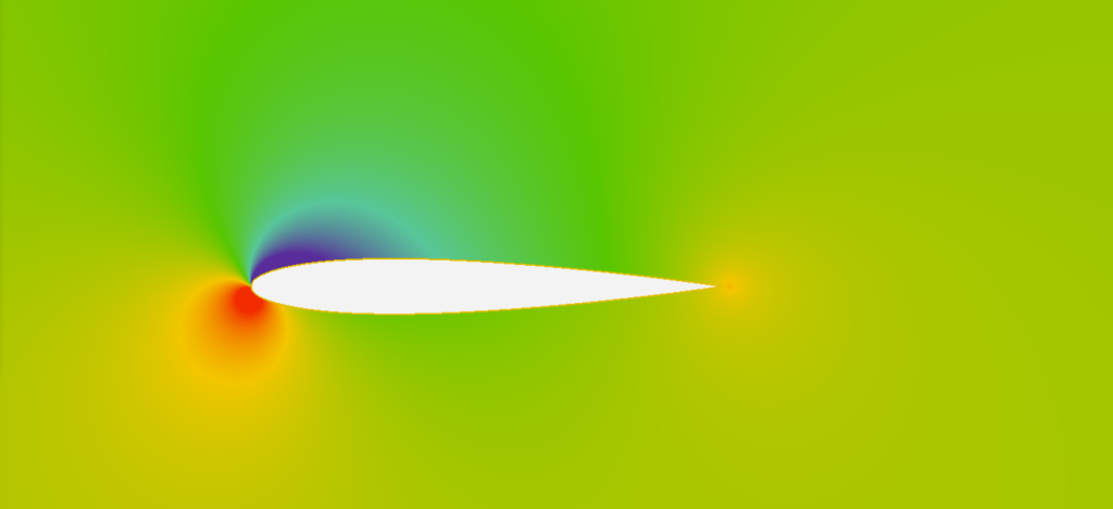
Velocity contour plot

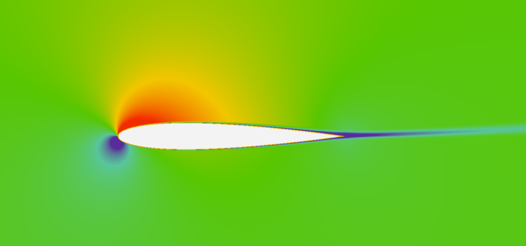
The velocit contour plot for the simulation with an angle of attack of $4^{\circ}$ is presented below.

Pressure contour plot

Effective lift generation can be observed by the high-pressure region on the lower surface and the low-pressure region on the upper surface.

Lift and drag

The simulation’s results for lift and drag as a function of angle of attack are compared to experimental data that can be found on the NASA website. When using the Spalart-Allmaras model, comparison with tripped data is usually preferred. In the tripped data, the boundary layer transition to turbulence is forced from the leading edge, which is consistent with the Spalart-Allmaras model’s ability to simulate fully turbulent flows.

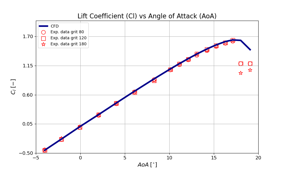
The comparison of lift coefficients from CFD and experimental data at various angles of attack reveals an exceptionally strong correlation. The Spalart-Allmaras turbulence model accurately captures the lift coefficient over almost the entire range. However, at very high angles of attack, where stall occurs, the model has difficulty accurately capturing the behaviour. It’s worth noting that this model is calibrated for small angles of attack, so predicting stall conditions is not its intended use.

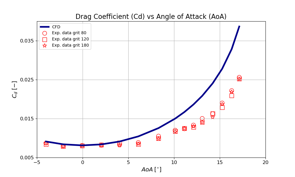
The drag coefficient presents a different story compared to the lift coefficient. The lift coefficient closely matches experimental data across nearly the entire range of angles of attack, whereas the drag coefficient deviates more. At small angles of attack, the drag estimation is consistent with experimental results. However, at larger angles, where flow detachment occurs, the turbulence model has difficulty accurately capturing the wake’s physics. In the wake region, the Spalart-Allmaras turbulence model can be overly dissipative.

Pressure coefficient

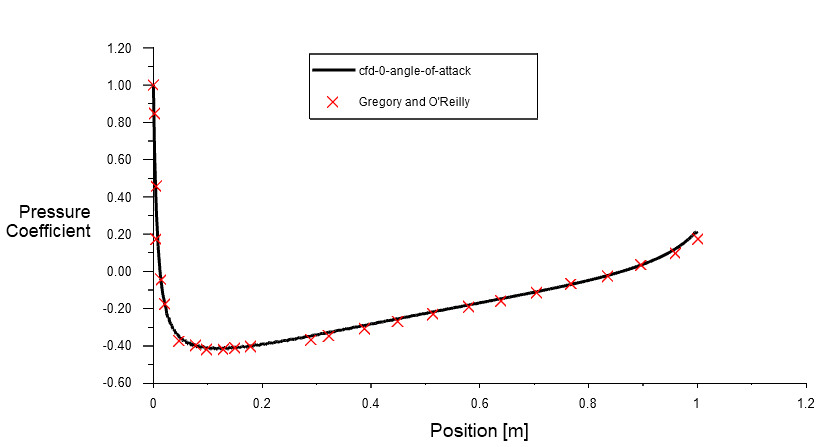
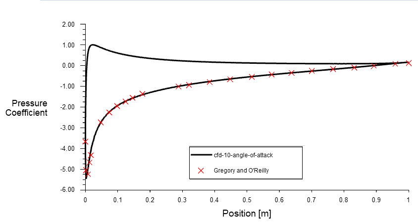
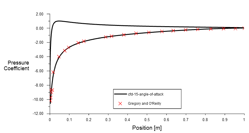
The pressure coefficient at different angles of attack is compared with experimental data in the figure below. This data, obtained at a Reynolds number of 2.88 million, is published on the NASA website. The pressure coefficient calculated using the Spalart-Allmaras turbulence model shows excellent agreement with the experimental data.

Conclusion

Boeing developed the model to optimise transonic lifting surfaces under cruise conditions. Within its intended scope, it is simple, robust, and accurate, especially at moderate angles of attack. However, its performance degrades near stall conditions due to the complex physics involved, such as laminar separation and turbulent reattachment. These phenomena exceed the model’s capabilities. The main takeaway is that, while simple turbulence models can be effective within validated parameters, their limitations become apparent when used outside of their intended application, necessitating careful interpretation of results.